
토치비전(torchvision)은 파이토치에서 제공하는 데이터셋들이 모여있는 패키지
- transforms: 전처리할 때 사용하는 메소드 (https://pytorch.org/docs/stable/torchvision/transforms.html)
- transforms에서 제공하는 클래스 이외는 일반적으로 클래스를 따로 만들어 전처리 단계를 진행
import torch
from torch.utils.data import Dataset,DataLoader
import torchvision.transforms as transforms
from torchvision import datasetsDataLoader의 인자로 들어갈 transform을 미리 정의할 수 있고, Compose를 통해 리스트 안에 순서대로 전처리 진행
ToTensor()를 하는 이유는 torchvision이 PIL Image 형태로만 입력을 받기 때문에 데이터 처리를 위해서 Tensor형으로 변환 필요
mnist_transform = transforms.Compose([transforms.ToTensor(),
                                      transforms.Normalize(mean=0.5,std=(1.0,))])
trainset= datasets.MNIST(root='/content/',
                         train=True,download=True,
                         transform=mnist_transform)
testset= datasets.MNIST(root='/content/',
                         train=False,download=True,
transform=mnist_transform)DataLoader는 데이터 전체를 보관했다가 실제 모델 학습을 할 때 batch_size 크기만큼 데이터를 가져옴
train_loader = DataLoader(trainset,batch_size=8,shuffle=True,num_workers=2)
test_loader = DataLoader(testset,batch_size=8,shuffle=False,num_workers=2)dataiter = iter(train_loader)
images, labels = next(iter(train_loader))
images.shape, labels.shape #28*28이미지, 1은 흑백 , 즉 8개의 흑백사진(torch.Size([8, 1, 28, 28]), torch.Size([8]))torch_image = torch.squeeze(images[0]) #차원 축소
torch_image.shape #1*28*28 하나만 가져와서 앞의 차원(1) 버림torch.Size([28, 28])import matplotlib.pyplot as plt
figure = plt.figure(figsize=(12,6))
cols,rows = 4,2
for i in range(1,cols*rows+1):
sample_idx= torch.randint(len(trainset),size = (1,)).item() #전체 길이 length 값에 대해서 random값을 가져오되 실제값을 인덱스로 사용
img,label = trainset[sample_idx]
figure.add_subplot(rows,cols,i)
plt.title(label)
plt.axis('off')
plt.imshow(img.squeeze(),cmap='gray')
plt.show() #이미지 넣고 숫자 맞추기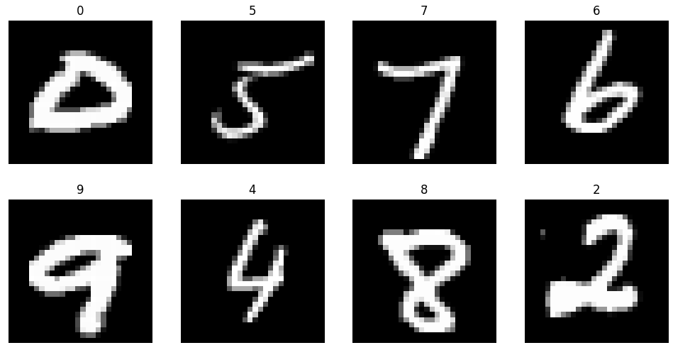
신경망 구성
- 레이어(layer): 신경망의 핵심 데이터 구조로 하나 이상의 텐서를 입력받아 하나 이상의 텐서를 출력
- 모듈(module): 한 개 이상의 계층이 모여서 구성
- 모델(model): 한 개 이상의 모듈이 모여서 구성
torch.nn 패키지
주로 가중치(weights), 편향(bias)값들이 내부에서 자동으로 생성되는 레이어들을 사용할 때 사용 (weight값들을 직접 선언 안함)
import torch.nn as nn
input = torch.randn(128,20)
print(input)

m = nn.Linear(20,30) #입력되는 feature, output feature 30  입력 텐서의 각 데이터 포인트가 20차원에서 30차원으로 변환

output = m(input) #input을 선형변환
print(output)
print(output.size())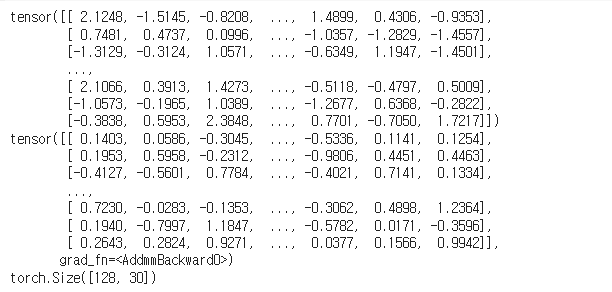
nn.Conv2d 계층 예시
input = torch.randn(20,16,50,100)
print(input.size())torch.Size([20, 16, 50, 100])
m = nn.Conv2d(16,33,3,stride=2)
m = nn.Conv2d(16,33, (3,5),stride=(2,1),padding=(4,2))
m = nn.Conv2d(16,33,(3,5),stride=(2,1),padding=(4,2),dilation=(3,1))
#16개 입력채널 33개 출력채널 (3,5) 합성곱 커널 크기 , dilation 합성곱 커널 내의 각 원소 사이의 간격을 조절하는 인자
print(m)Conv2d(16, 33, kernel_size=(3, 5), stride=(2, 1), padding=(4, 2), dilation=(3, 1))l
output = m(input)
print(output.size()) #out channels 따라서 지정torch.Size([20, 33, 26, 100])
컨볼루션 레이어(Convolution Layers)
nn.Conv2d 예제
- in_channels: channel의 갯수
- out_channels: 출력 채널의 갯수
- kernel_size: 커널(필터) 사이즈
nn.Conv2d(in_channels=1,out_channels=20,kernel_size=5,stride=1)Conv2d(1, 20, kernel_size=(5, 5), stride=(1, 1))layer = nn.Conv2d(1,20,5,1).to(torch.device('cpu'))
layer #cpu로 전송Conv2d(1, 20, kernel_size=(5, 5), stride=(1, 1))weight 확인
weight = layer.weight
weight.shapetorch.Size([20, 1, 5, 5])weight는 detach()를 통해 꺼내줘야 numpy()변환이 가능
weight = weight.detach()
weight = weight.numpy()
weight.shape(20, 1, 5, 5)plt.imshow(weight[0,0,:,:],'jet')
plt.colorbar()
plt.show()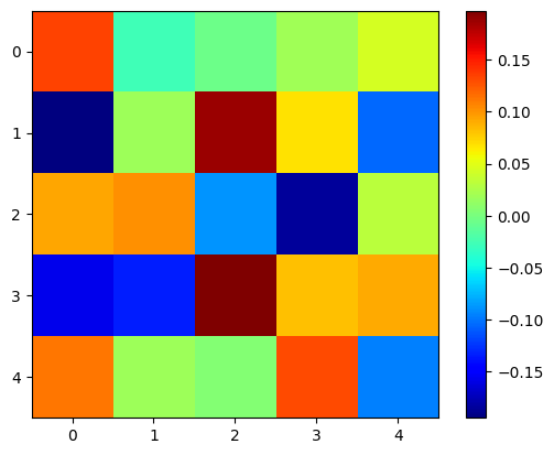
print(images.shape)
print(images[0].size())
input_image = torch.squeeze(images[0])
print(input_image.size())torch.Size([8, 1, 28, 28])
torch.Size([1, 28, 28])
torch.Size([28, 28])
input_data = torch.unsqueeze(images[0],dim=0)
print(input_data.size())

output_data = layer(input_data)
output = output_data.data
output_arr = output.numpy()
output_arr.shape  #흑백사진 한장, layer통과시킨것에 대해 데이터만 뽑아서 numpy 변환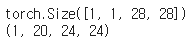
plt.figure(figsize=(15,30))

plt.subplot(131)
plt.title('input')
plt.imshow(input_image,'gray')

plt.subplot(132)
plt.title('Weight')
plt.imshow(weight[0,0,:,:],'jet')

plt.subplot(133)
plt.title('Output')
plt.imshow(output_arr[0,0,:,:],'gray')
plt.show() #covlyer 가중치 통과했을 떄 나오는 output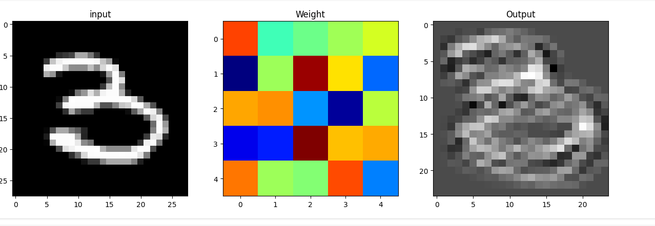
풀링 레이어(Pooling layers)
- F.max_pool2d
- stride
- kernel_size
- torch.nn.MaxPool2d 도 많이 사용
import torch.nn.functional as F
pool = F.max_pool2d(output,2,2) #2개를 기준으로 max값만 지정해줘, 가로세로 반으로 줄어듦
pool.shapetorch.Size([1, 20, 12, 12])- MaxPool Layer는 weight가 없기 때문에 바로 numpy()변환 가능
pool_arr = pool.numpy()
pool_arr.shape(1, 20, 12, 12)plt.figure(figsize=(10,15))
plt.subplot(131)
plt.title('input')
plt.imshow(input_image,'gray')
plt.subplot(132)
plt.title('Output')
plt.imshow(pool_arr[0,0,:,:],'gray') #해상도가 반으로 줄어들음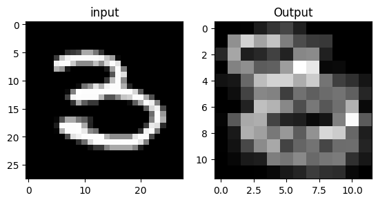
선형 레이어(Linear layers)
1d만 가능하므로 .view()를 통해 1d로 펼쳐줘야함
flatten  = input_image.view(1,28*28)
flatten.shapetorch.Size([1, 784])lin = nn.Linear(784,10)(flatten)#in_feature 784, out 10
lin.shapetorch.Size([1, 10])lin #10개tensor([[ 0.0827, -0.0323, -0.0230, -0.3806, 0.0301, 0.2720, -0.1341, -0.1413,
0.0194, 0.0713]], grad_fn=<AddmmBackward0>)plt.imshow(lin.detach().numpy(),'jet')
plt.colorbar()
plt.show()
#10개의 값 출력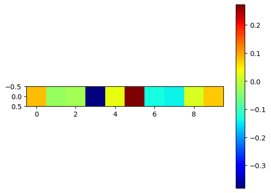
비선형 활성화 (Non-linear Activations)
F.softmax와 같은 활성화 함수 등
with torch.no_grad():
  flatten  = input_image.view(1,28*28)
  lin = nn.Linear(784,10)(flatten)
  softmax= F.softmax(lin,dim=1)

softmaxtensor([[0.0587, 0.0785, 0.1172, 0.1054, 0.1060, 0.1078, 0.1148, 0.0918, 0.1187,
0.1009]])import numpy as np
np.sum(softmax.numpy()) #10개의 합1.0F.relu
- ReLU 함수를 적용하는 레이어
- nn.ReLU로도 사용 가능
device = torch.device('cuda' if torch.cuda.is_available()  else 'cpu')
input = torch.randn(4,3,28,28).to(device)
input.shapetorch.Size([4, 3, 28, 28])layer = nn.Conv2d(3,20,5,1).to(device) #conv layer 통과
output = F.relu(layer(input))#act function 지
output.shapetorch.Size([4, 20, 24, 24])
출처: https://youtu.be/k60oT_8lyFw?si=mkFA_BBlxHgcmc2Q
'Python' 카테고리의 다른 글
| 클래스 (0) | 2024.03.31 |
|---|---|
| pytorch 이미지 모델링 II (1) | 2024.02.26 |
| pytorch 기본문법 II (1) | 2024.02.24 |
| pytorch 기본 문법 I (1) | 2024.02.24 |
| Window 11 python tensorflow gpu 설치 (1) | 2023.11.12 |